Investigating junctions further: positions and sequences

Using summary statistics, in the previous part of the tutorial we have singled out a junction we want to investigate further. Here we will showcase the use of two BackboneJunctions methods for this:

• positions(): indicates the location of each occurrence of the junction on the genomes that carry it. Useful e.g. for cross-referencing with annotation files.
• sequences(): returns the actual DNA sequence spanning the junction on every genome, as Bio.SeqRecord objects ready to be written to FASTA for further analysis (multiple sequence alignment, secondary pangraph construction, BLAST searches, ...).

The example: a candidate IS insertion

As a running example we will use the same junction introduced in the previous section: the edge 10485686697184953244_r__1548999589339136461_f. Looking up its row in the statistics dataframe:

import pypangraph as pp

graph = pp.Pangraph.from_json("staph.json.gz")
junctions = pp.junctions.BackboneJunctions(graph, L_thr=500)
stats = junctions.stats()

edge = "10485686697184953244_r__1548999589339136461_f"
print(stats.loc[edge])
# n_isolates                15
# n_non_empty                1
# n_categories               2
# accessory_length        1324
# ...

We found multiple junctions with this specific accessory length and low number of non-empty paths, indicative of a putative recent Insertion Sequence (IS) insertion.

Genomic coordinates of a junction

The positions() method returns a pandas.DataFrame indexed by (edge, isolate), with the genomic coordinates of the two flanking core blocks plus a strand flag. We slice on our edge of interest with .loc:

all_positions = junctions.positions()
junction_pos = all_positions.loc[edge]
print(junction_pos)
#                left_start  left_end  right_start  right_end  strand
# iso                                                                
# NZ_CP132362.1     2509902   2511822      2511822    2516373   False
# NZ_LR822061.1     1288340   1290278      1290278    1294829   False
# NZ_CP077852.1     1661385   1665936      1665936    1667856    True
# ...
# NZ_CP169947.1      880245    884796       884796     886716    True
# NZ_CP022905.1      872983    877542       878866     880786    True
# NZ_CP035791.1     1215039   1216959      1216959    1221510   False

The columns are:

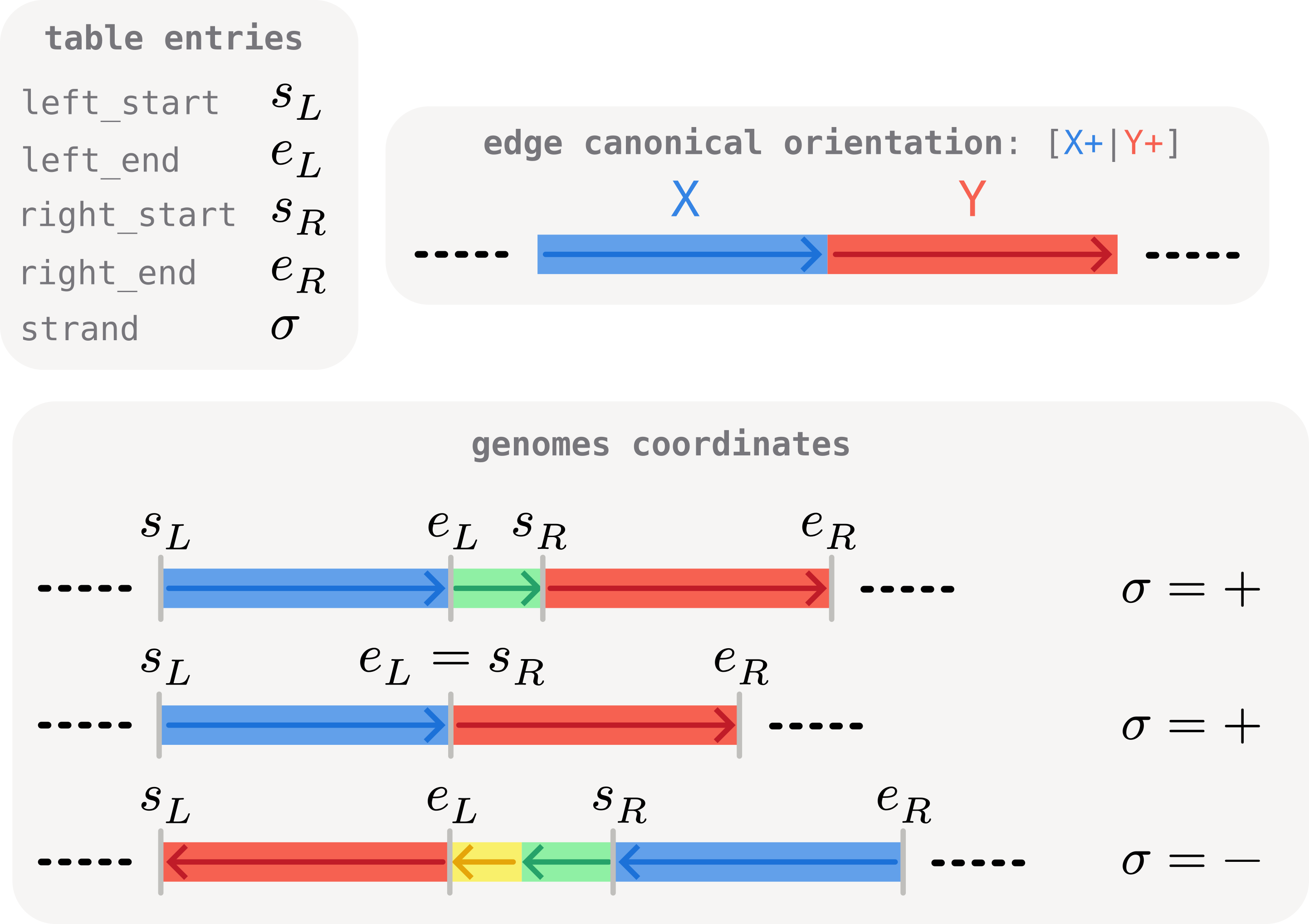
• left_start, left_end: genomic coordinates of the left flanking core block on the genome.
• right_start, right_end: genomic coordinates of the right flanking core block on the genome.
• strand: True if the junction appears in canonical edge orientation on this genome, False if reverse-complemented.

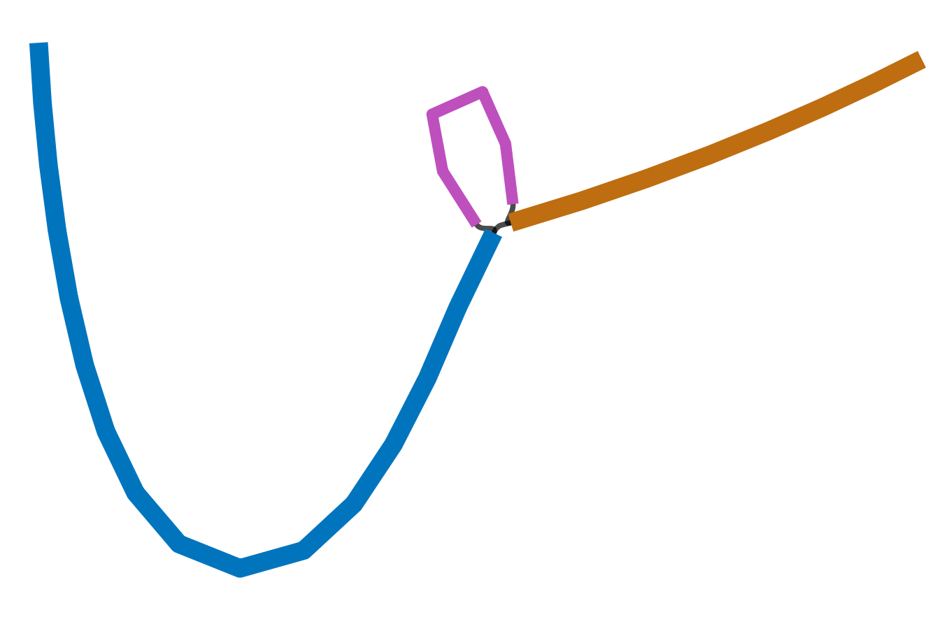
Note that the left / right labels follow each genome's own path order: the left block is the first core block of the junction encountered when walking the genome, as illustrated in the scheme below. On isolates where the junction path is inverted (strand = False), this means the left/right roles are swapped relative to the canonical edge direction.

The coordinates on the genome should therefore always satisfy left_start < left_end < right_start < right_end, irrespective of orientation. In circular genomes there can be exceptions to this pattern, as described below.

circular genomes

In circular genomes, a junction path might wrap around the genome origin. In such cases the left core block might be found around the end of the sequence, and the right core block at the beginning. As such, in these genomes the order of positions described will not be respected.

The difference between the left_end and right_start coordinates gives the precise size of the accessory region. This is zero when no accessory blocks are present.

junction_pos.eval("right_start - left_end")
# iso
# NZ_CP132362.1       0
# NZ_LR822061.1       0
# NZ_CP077852.1       0
# ...
# NZ_CP169947.1       0
# NZ_CP022905.1    1324  <-- IS insertion
# NZ_CP035791.1       0

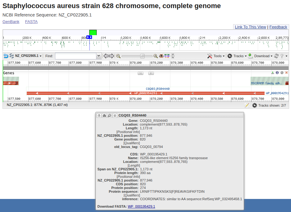
As we saw in the linear representation of the junction in the previous tutorial section, the insertion is only present in genome NZ_CP022905.1 between coordinates:

junction_pos.loc["NZ_CP022905.1", ["left_end", "right_start"]]
# left_end       877542
# right_start    878866

Inspecting this location in NCBI's GenBank viewer reveals indeed the presence of an IS256 element, commonly found in S. aureus, and likely to have recently inserted and given rise to the junction.

The location of an insertion is often not random. If inserted in a coding region, an IS element can have significant fitness effects by disrupting genes. We can easily check if this is the case for our insertion by observing whether the junction breakpoint falls in a coding region in genomes where the IS element is absent. For example, consulting the pos table above, we can check genome NZ_LR822061.1 at coordinate 1290278.

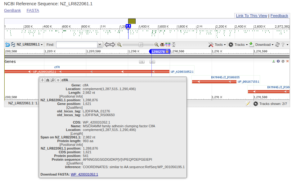
The IS element insertion truncates the clfA gene, which encodes an immunogenic surface protein involved in adhesion, a known virulence factor.

Extracting the junction sequences

For further downstream analysis you often want the nucleotide sequence of a junction. The sequences() method returns one Bio.SeqRecord per isolate, spanning left flank + accessory center + right flank, all co-oriented to the canonical edge direction so that no further inversion is necessary.

records = junctions.sequences(edge)
for r in records:
    print(f"{r.id}: {r.seq[:10]}...{r.seq[-10:]} | len = {len(r.seq)} bp")
# NZ_CP132362.1: ATTTGTAGCC...ACTCAGACAG | len = 6471 bp
# NZ_LR822061.1: ATTTGTAGCC...ACTCAGACAG | len = 6489 bp
# NZ_CP077852.1: ATTTGTAGCC...ACTCAGACAG | len = 6471 bp
# ...
# NZ_CP169947.1: ATTTGTAGCC...ACTCAGACAG | len = 6471 bp
# NZ_CP022905.1: ATTTGTAGCC...ACTCAGACAG | len = 7803 bp
# NZ_CP035791.1: ATTTGTAGCC...ACTCAGACAG | len = 6471 bp

The IS carrier (NZ_CP022905.1) stands out as ~1.3 kb longer than the rest. Each record has:

• id: the isolate name.
• description: the canonical edge string.
• seq: the DNA from the start of the left flank to the end of the right flank.

These can be conveniently exported in a fasta file using biopython for further downstream processing.

from Bio import SeqIO

SeqIO.write(records, "junction.fa", "fasta")

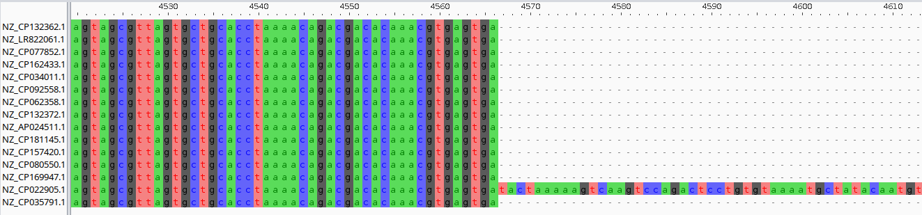
For example a multiple sequence alignment with MAFFT:

mafft junction.fa > junction_aligned.fa

Or a second, junction-specific pangraph. This is usually useful in more complex junctions, to refine the junction structure.

pangraph build -l 100 -s 20 junction.fa -o junction.json
pangraph export gfa junction.json -o junction.gfa

More junctions to explore

As a further exercise you can try to explore some more interesting junctions yourself. Here are some suggestions:

• look into 13654622636097204630_f__5922465870918455593_f.
  • Can you locate the prophage insertion?
  • Find its coordinates in the genome and visualize it on NCBI. Inspecting the annotations of the accessory region should confirm that it is likely a prophage integration. Where did it get integrated? Note: it wraps around the start of the sequence record.
  • Can you find the gene immediately upstream of the prophage insertion and the first gene of the accessory region? Does this suggest a mechanism of integration?
• edge 10486523597117694808_f__6531151666869853507_r is another simple example of a junction originated by an IS element insertion.
  • Which gene is inactivated by the insertion? Take one of the isolates without the insertion (e.g. NZ_CP132362.1) and check which gene is present at the location where isolate NZ_LR822061.1 shows an insertion. You should find that the insertion likely inactivated the staphylocoagulase, a known virulence factor.
  • This is just one example of gene inactivation; in the junction overview plot we noted that several junctions originated from an IS movement. What is the general pattern? Can you automate this search and check how often a recent IS element insertion interrupted a gene? Is this more or less frequent than what is expected by chance? What could be the selective forces driving this imbalance?
• look into 17042526223432838337_f__8287974428665837959_r
  • Can you spot a duplication in some sequences? Which genes are duplicated?
• edge 13256234721607664913_r__7427484406751306657_f encompasses a highly-variable region in these genomes.
  • draw a linear representation to compare the variation across different genomes.
  • focus on one genome, e.g. NZ_CP022905.1, and look at the annotations. Can you find mobile genetic elements? Can you find resistance determinants?
  • the presence of the mecA gene and recombinases suggests that this is a SCCmec cassette (IWG-SCC 2009), a known mobile genetic element of Staphylococcus bacteria that confers methicillin resistance.