Junctions: comparing local accessory variation

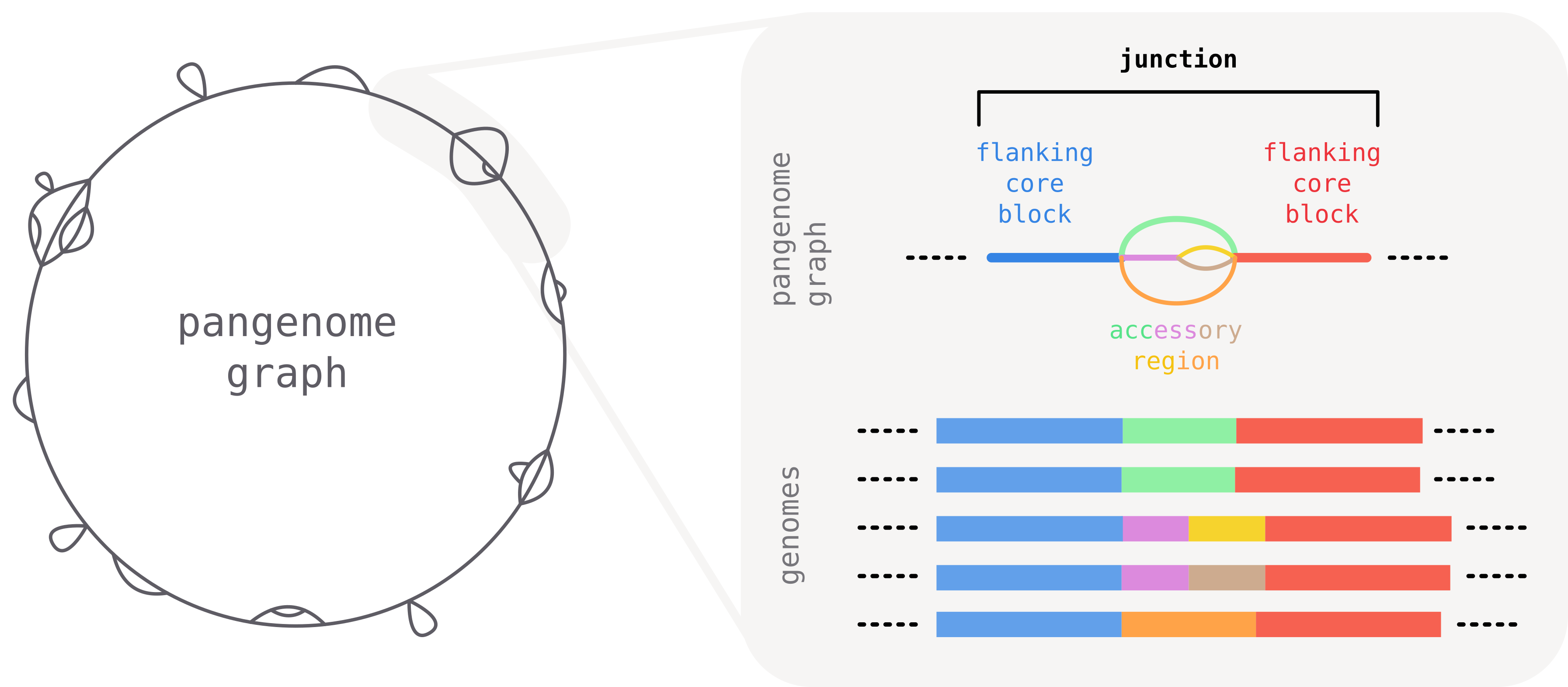
When comparing closely related bacterial genomes, the core genome is often largely syntenic: long stretches of conserved blocks appear in the same order across isolates. Between these conserved blocks, segments of accessory DNA (insertions, deletions, mobile elements) vary from one genome to another.

The largely conserved order of core segments provides a natural frame of reference to meaningfully break down and compare local accessory variation across isolates. To this end we introduce the concept of a junction: a region of the graph delimited by two consecutive core blocks.

What is a junction?

A junction is defined as the part of the graph "between" two consecutive core-blocks. It starts and ends with the two flanking core blocks that serve as anchor points, and contains all accessory diversity in-between.

Unique identifiers for junctions: core edges

A graph can contain a large number of junctions, but each is uniquely defined by the two flanking core blocks. Their identity and orientation determines the identity of the junction.

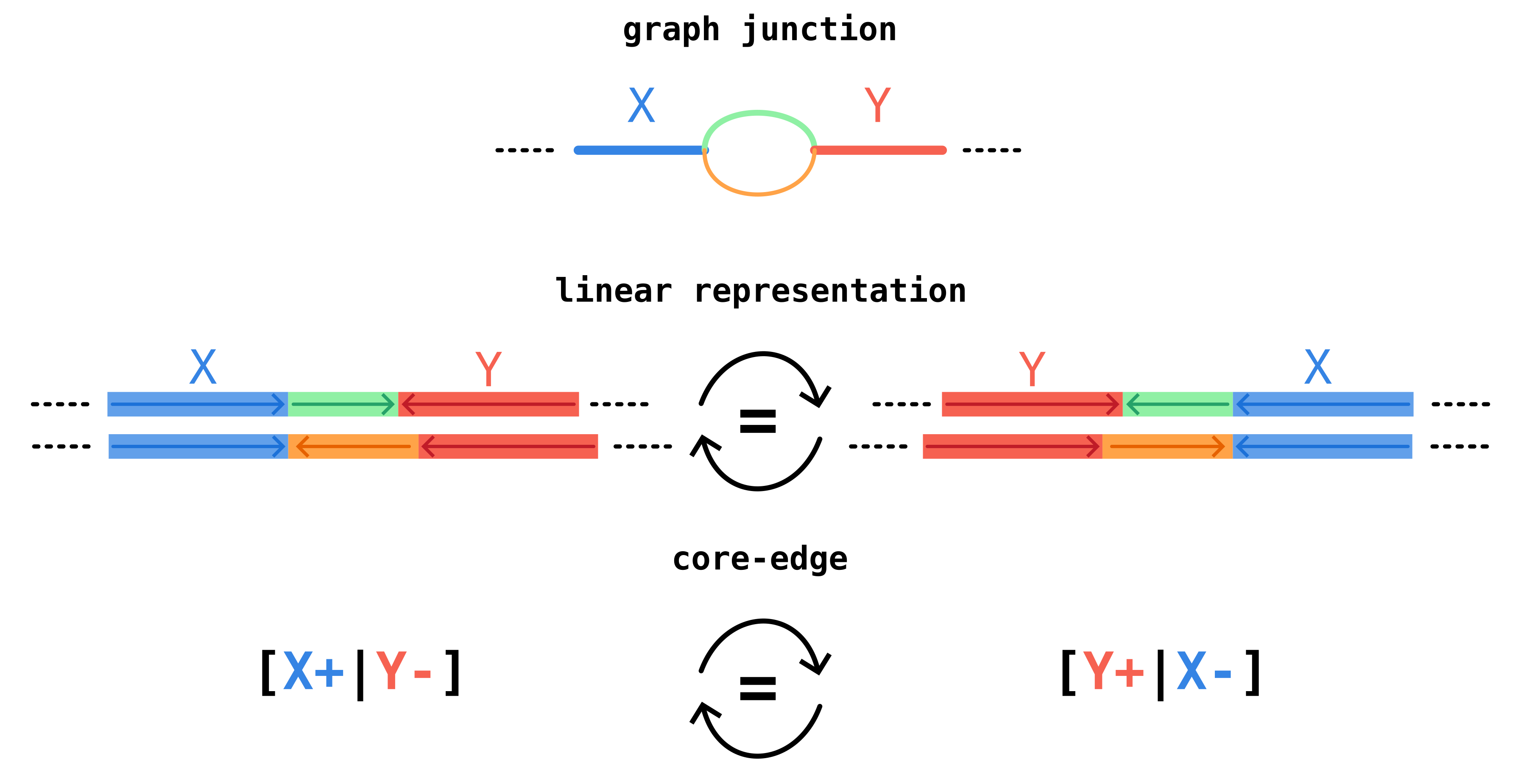
We call a core edge the oriented adjacency relation of two core blocks, neglecting accessory blocks in-between. In the example below, core blocks X and Y form a core edge with orientation [X+|Y-].

This notation indicates that in genomes we observe first a sequence homologous to the consensus sequence of block X (denoted as X+) and then (potentially after an accessory region) a sequence homologous to the reverse complement of the consensus sequence of block Y (denoted as Y-).

The same junction region can occur with different strandedness on different genomes, but it should still be identified as the same junction. For this reason we define core-edges to be invariant under reverse-complementation, so [X+|Y-] and its reverse complement [Y+|X-] correspond to the same core edge.

In pypangraph core edges are identified by a string of the form X_a__Y_b, where X and Y are large integers corresponding to the block_id of the two blocks, and a and b are either f or r, indicating respectively forward (+) or reverse (-) orientation.

Since edges are equivalent under reverse-complementation, there are actually two possible strings that can identify an edge. To break the tie we take the lexicographically smaller. This order defines the canonical orientation of the junction.

The junctions module in pypangraph

Pypangraph has a junctions module to facilitate junction analyses.

In this part of the tutorial we will load and explore the staph.json.gz file, which contains a pangraph of 15 Staphylococcus aureus chromosomes. You can download it from the pypangraph repository at packages/pypangraph/tests/data/staph.json.gz.

how was staph.json.gz built?

The graph was built from 15 complete S. aureus chromosomes downloaded from NCBI. To reproduce it, fetch the sequences and run pangraph build:

ACCESSIONS="NZ_CP132362.1,NZ_LR822061.1,NZ_CP077852.1,NZ_CP162433.1,NZ_CP034011.1,NZ_CP092558.1,NZ_CP062358.1,NZ_CP132372.1,NZ_AP024511.1,NZ_CP181145.1,NZ_CP157420.1,NZ_CP080550.1,NZ_CP169947.1,NZ_CP022905.1,NZ_CP035791.1"

# download the sequences in FASTA format
curl -L "https://eutils.ncbi.nlm.nih.gov/entrez/eutils/efetch.fcgi?db=nuccore&id=${ACCESSIONS}&rettype=fasta&retmode=text" > staph.fa

# build the pangraph
pangraph build --circular -l 100 -s 20 -b 5 staph.fa -o staph.json.gz

We start by loading the graph and creating a BackboneJunctions object. This class identifies junctions in the graph and provides methods to analyze them.

import pypangraph as pp

graph = pp.Pangraph.from_json("staph.json.gz")
print(graph)
# pangraph object with 15 paths, 664 blocks and 6817 nodes

junctions = pp.junctions.BackboneJunctions(graph, L_thr=500)

The constructor takes only two arguments: the graph object and a length threshold L_thr (default 500 bp). Core blocks shorter than this threshold are too short to be reliable anchors and are treated as accessory blocks for the purpose of junction definition.

A look at edges

The graph has a total of 143 valid anchor core blocks.

graph.to_blockstats_df().query("len >= 500")["core"].sum()
# 143 core blocks

We can get the list of edges with:

print(junctions.edges())
# ['13733442150340492168_f__17042526223432838337_f',
#  '12427448985183016017_f__13733442150340492168_f',
#  '12427448985183016017_r__14846644350907526570_f',
#  '11809679528571820295_f__14846644350907526570_r',
#  ...
# ]
# a total of 151 edges

There are 151 edges, which is only slightly more than the number of core blocks. This means that, as expected, the order of core blocks is strongly conserved and almost every core block has the same core block neighbors in every genome. Across the whole dataset we expect to observe only a handful of synteny changes.

Selecting a junction and a single path through it

To get a feel for what a junction actually looks like, let's pick one and inspect it. Indexing into the BackboneJunctions object by edge id returns the {isolate: Junction} mapping for that edge; a second index by isolate name gives the path of a single isolate through the junction:

# core edge
edge_str = "3156970751805415521_f__4335229004353524956_f"
# select the junction corresponding to that edge
junction = junctions[edge_str]
# select the path of a single isolate through that junction
junction_path = junction["NZ_CP162433.1"]

Each junction path contains the left flanking core block, the center walk of accessory blocks, and the right flanking core block, accessible as attributes:

print(junction_path.left)
# {block=4335229004353524956|-}
print(junction_path.right)
# {block=3156970751805415521|-}
print(junction_path.center)
# {block=8061287138899943998|-} {block=12150994386844653378|-}
print(len(junction_path.center))
# 2

Each block occurrence is printed as {block=<block_id>|<strand>}.

Note that both flanking blocks appear on the reverse strand (-) and in swapped order with respect to the canonical edge ID we asked for (3156970751805415521_f__4335229004353524956_f). This is the reverse-complement symmetry introduced earlier: this isolate carries the junction in its reverse orientation, but the edge ID (the canonical, orientation-invariant identifier) is the same.

Next: from a single junction to summary statistics

Inspecting individual junctions like the one above gives a concrete sense of what a junction is, but a graph contains hundreds of them, and going through one at a time quickly becomes impractical. To get an overview of the structural variation landscape, and to spot the junctions worth zooming in on, we need summary statistics across all junctions. This will be the focus of the next part of the tutorial.