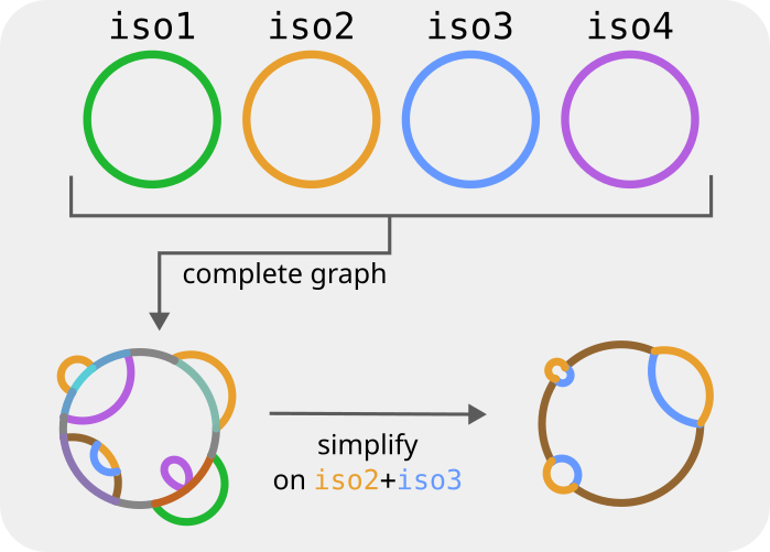
Projecting the graph on a subset of strains.

In this next part of the tutorial we show how to use the simplify command. This command is used when one is interested in the relationship between a subset of the genomes that make up the pangraph. It can quickly create, starting from the full pangraph, a smaller pangenome graph relative to the selected subset of strains.

Preliminary steps

We will run this tutorial on a different dataset, containing 9 complete chromosomes of Klebsiella Pneumoniae (source: GenBank). These sequences are available in the pangraph repository (example_dataset/klebs.fa.gz) and can be downloaded by running:

curl https://github.com/neherlab/pangraph/raw/master/example_datasets/klebs.fa.gz

As for the previous dataset, we can create the pangraph with the command:

pangraph build --circular -j 4 klebs.fa.gz -o klebs_pangraph.json

On 4 cores the command should complete in around 4 mins using 4 threads. After creating the pangraph, we can export it in gfa format for visualization.

pangraph export gfa \
    --no-duplicated \
    klebs_pangraph.json \
    -o klebs_pangraph.gfa

The output file can be visualized using Bandage.

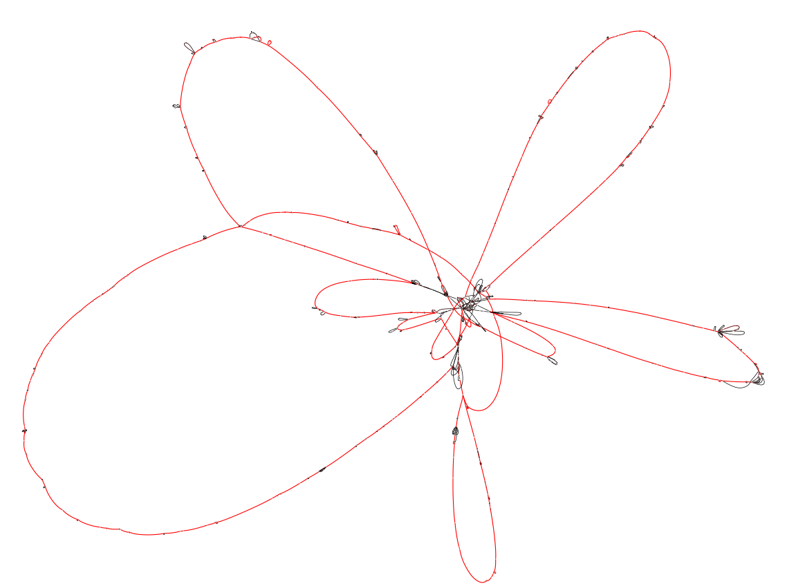
Colors indicate the number of times a block occurs. Blocks that appear in red are core blocks that are found in every chromosome, while black blocks are only present in a few strains. We used the --no-duplication flag in the export command, which excludes duplicated blocks from the exported graph. This simplifies the visualization, which would otherwise be highly "tangled-up" by these duplications.

Marginalize the graph on a subset of strains

The full graph might be difficult to interpret. However if we are interested only in relationships between a subset of chromosomes we can use the command simplify to project the pangraph on this set of strains. This "simplification" operation will remove transitive edges. If two blocks always come one after the other (with same strandedness) in all of the subset of strains one is interested in, these blocks will be merged in a new larger block. This can greatly simplify the pangenome graph, and highlight differences between a particular subset of strains. And it is also computationally much faster than building a new pangraph directly from the sequences of interest.

For this example we will consider the pair of strains NZ_CP013711 and NC_017540.¹ We can marginalize the pangraph on these two strains by running:

pangraph simplify \
    klebs_pangraph.json \
    --strains='NZ_CP013711,NC_017540' \
    -o klebs_marginal_pangraph.json

The file klebs_marginal_pangraph.json will contain the new marginalized pangraph. The strains on which one projects are specified with the flag --strains. They must be passed as a comma separated list of sequence ids, without spaces.

options and positional arguments

Make sure you handle options and positional arguments correctly: if an option requires a value and you don't provide it, the positional argument following the option could be incorrectly treated as the options' value, due to ambiguity in parsing:

pangraph --option <forgot_the_value_here> positional_arg

Also, consider using --option=value syntax as well as end-of-options delimiter (--) to disambiguate:

pangraph --option=value -- positional_arg

A look at the marginalized pangraph

As done for the main pangraph, we can export the marginalized pangraph in gfa format:

pangraph export gfa \
    --no-duplications \
    --minimum-length 150 \
    klebs_marginal_pangraph.json \
    -o klebs_marginal_pangraph.gfa

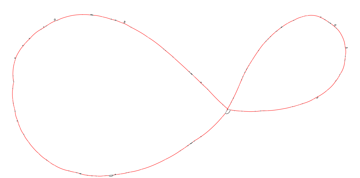
As expected the marginalized pangraph contains fewer blocks than the original one (388 vs 1244), and blocks are on average longer (mean length: 14 kbp vs 6 kbp). Blocks that appear in red are shared by both strains, while black blocks are present in only one of the two strains. The pangraph is composed of two stretches of syntenic blocks, which are in contact in a central point. This structure can be understood by comparing the two chromosomes with a dotplot (see dotplots with pypangraph)

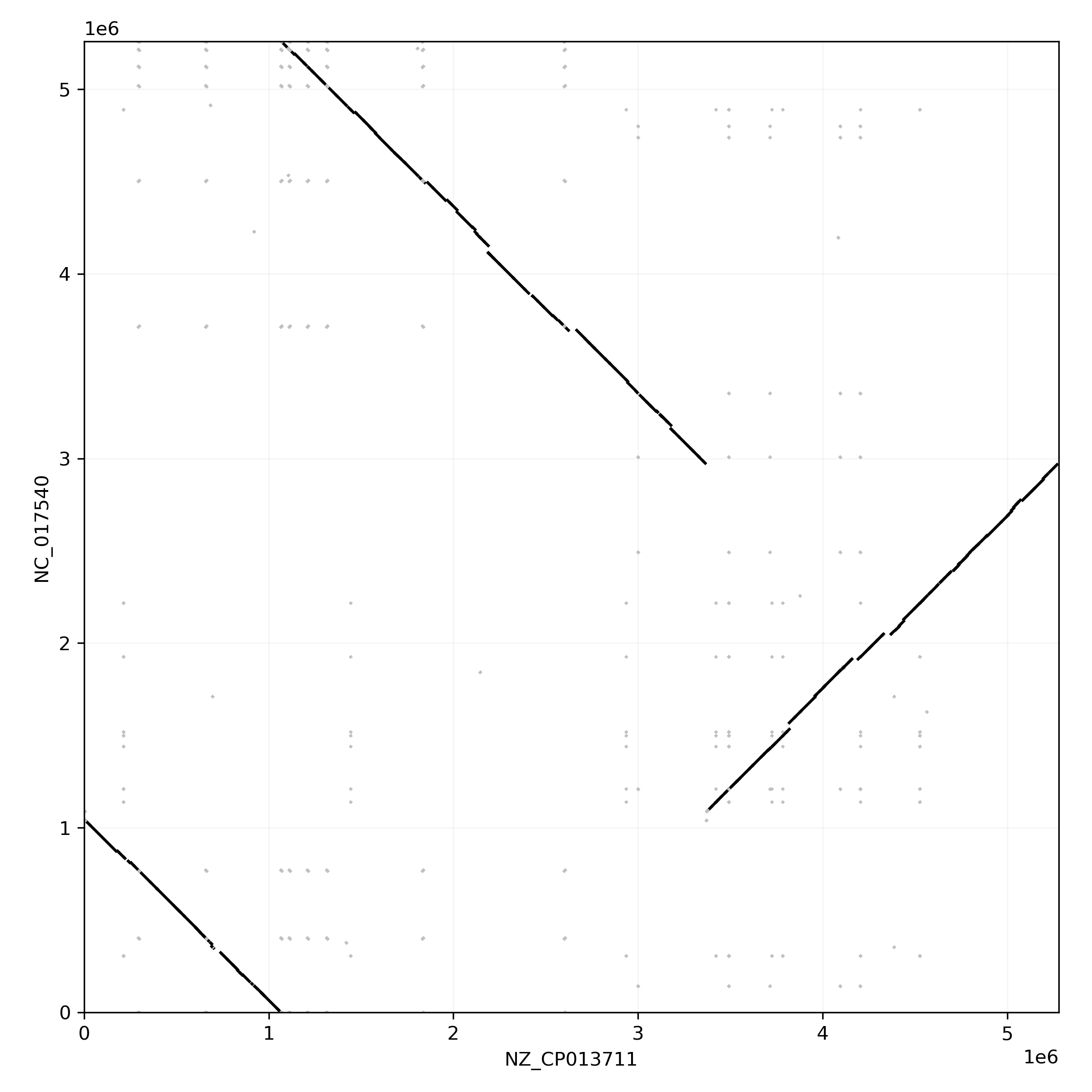
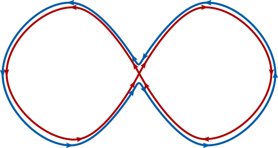
The contact point between the two loops in the pangraph is caused by the fact that the two genomes are composed of two mostly syntenic subsequences (the two loops) but these loops are concatenated with two different strandedness in the two strains. If we were to draw the two paths (relative to the two chromosomes) with different colors on top of the pangraph we would observe something similar to this:

Footnotes

1. here we consider a marginalization on two strains, but one can marginalize the pangraph on any number of strains. ↩